Predicting Electric Vehicle Range
See the full Jupyter Notebook on GitHub.
Electric vehicles are rapidly gaining in popularity. Electric vehicle registrations have jumped at least 23% over the past four years, and currently make up about 5.5% of the market. One of the major drawbacks (and concerns from consumers) of electric vehicles is their range. Electric vehicles take much longer to charge than filling up a gas-powered vehicle and charging stations are still relatively rare.
In this project, we’ll take a look at an electric vehicle dataset to investigate predicting the range of each vehicle.
Data Set
We are using the Electric Vehicles data set from Kaggle. It contains information on 194 electric vehicles on the market until 2022.
Data Dictionary
id: unique identifierMake: brand of the carlink: source urlCity - Cold Weather: range in km under cold weather conditions (-10 deg) in citiesHighway - Cold Weather: range in km under cold weather conditions (-10 deg) on highwaysCombined - Cold Weather: range in km under cold weather conditions (-10 deg) combinedCity - Mild Weather: range in km under mild weather conditions (23 deg) in citiesHighway - Mild Weather: range in km under mild weather conditions (23 deg) on highwaysCombined - Mild Weather: range in km under mild weather conditions (23 deg) combinedAcceleration 0-100 km/h: acceleration from 0 to 100 km/hr in secondsTop Speed: top speed in km/hrElectric Range: advertised electric range in kmTotal PowerTotal TorqueDrive: Rear, Front, AWDBattery Capacity: total capacity of the battery in KWCharge PowerCharge SpeedFastcharge SpeedLength: car length in mmWidth: car width in mmHeight: car height in mmWheelbase: wheelbase in mmGross Vehicle Weight: gross weight of the car in kgMax PayloadCargo Volume: Cargo volume of the car in littersSeats: number of seats
Goal
Predict the Electric Range of the vehicle based on other vehicle properties.
Data Exploration
We will begin by loading the data and exploring it to get a better sense of the data set.
There are 24 columns and 194 rows as expected. There are 6 columns related to the range of the vehicle in different weather situations that contain similar, and possibly redundant information. These contain major data leakage, so we will drop these columns for our analysis.
Most of the columns have a variety of values. Charge Power and Seats both only have 5 unique values.
This data is very clean. This is great because we only have 194 rows of data. With such a small data set, we do not want to get rid of any data.
We have zero missing values. Nearly all of the values are already numerical. The Drive column is a categorical variable that contains only 3 values (AWD, Front, and Rear). The Make column is a categorical variable that has 34 unique values. The link column is a web link that does not provide useful information.
Visualizing the Data
Now, let’s create a few simple visualizations to further understand our data set. We start by plotting a histogram of every numerical column.
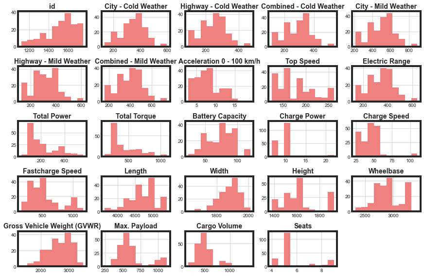
Max. Payload and Cargo Volume are clearly bimodal distributions. We’ll convert these to Low and High categories to reduce some of the complexity of our data set for our model. Top Speed could be dealt with similarly, but that option is less clear for that feature. Seats also only has 4 discrete options. The other distributions do not show any usual behavior that we will need to be concerned about.
Next, we will plot a diagonal correlation matrix to look for collinearity.
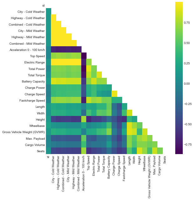
Since our target feature will be Electric Range, we can also calculate correlation coefficients with that column only.
| Column | Correlation Coefficient with Range |
|---|---|
| Acceleration 0 - 100 km/h | -0.708172 |
| Height | -0.540106 |
| Seats | -0.500843 |
| Max. Payload | -0.373626 |
| Cargo Volume | -0.145220 |
| Wheelbase | 0.061227 |
| id | 0.128289 |
| Length | 0.219826 |
| Gross Vehicle Weight (GVWR) | 0.269258 |
| Width | 0.277975 |
| Charge Power | 0.398395 |
| Charge Speed | 0.415019 |
| Total Torque | 0.614073 |
| Total Power | 0.637401 |
| Fastcharge Speed | 0.701595 |
| Top Speed | 0.706707 |
| Battery Capacity | 0.863062 |
| City - Cold Weather | 0.995611 |
| City - Mild Weather | 0.998262 |
| Highway - Mild Weather | 0.998401 |
| Highway - Cold Weather | 0.999215 |
| Combined - Cold Weather | 0.999298 |
| Combined - Mild Weather | 0.999340 |
The heat map and correlation table help us to start to identify which features we will want to keep for our modeling, and to identify any collinear features. Acceleration, Height, and Seats are all strongly anti-correlated with Electric Range. Total Torque, Total Power, Fastcharge Speed, Top Speed, and Battery Capacity are all strongly correlated with Electric Range.
Finally, let’s create a box plot for the Make column with the Electric Range target. This might help us understand if there is a way to utilize this feature.
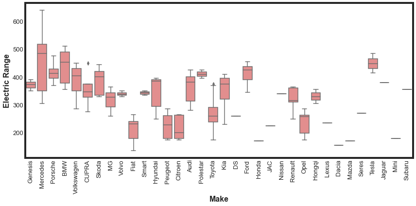
It could be that some vehicle makers prioritize range over other factors. However, our box plot does not show this clearly. With multiple makers only having a single car on the marker, we would have to also be careful with that skewing our expectations. For now, we will plan to not include Make in our modeling.
Data WorkFlow
Now, we are going to write a few functions that we will use repeatedly to prepare our data for modelling. These will allow us to quickly test and iterate. These functions will:
- remove unnecessary columns
- convert categorical columns to numerical
- engineer features
- convert numerical column to categorical
Our function to remove columns is:
def remove_columns(df,cols):
    '''Removes columns from dataframe and returns new dataframe

    INPUT
        df: dataframe
        cols: list, columns to remove

    OUTPUT
        reduced_df: dataframe with specified columns removed
    '''
    reduced_df = df.drop(cols,axis=1)
    return reduced_df
Our function to convert categorical columns to numeric is:
def process_categorical(df,column_name):
    '''Performs One Hot Encoding on categorical columns

    INPUT
        df: dataframe
        column_name: categorical column to convert to numerical

    OUTPUT
        processed_df: dataframe with specified columns removed
    '''
    dummies = pd.get_dummies(df[column_name],prefix=column_name)
    processed_df = pd.concat([df,dummies],axis=1)
    return processed_df
Our function to create a new density column is:
def engineer_density(df):
    '''Engineers a new feature for modelling, the density of the vehicle.
    INPUT
        df: dataframe

    OUTPUT
        df: dataframe with new feature
    '''
    df['volume'] = df['Height'] * df['Length'] * df['Width']
    df['density'] = df['Gross Vehicle Weight (GVWR)'] / df['volume']

    return df
And finally, our function to convert numerical columns to categorical is:
def make_categorical(df,col,new_col,cut_points,label_names):
    ''' Takes a numerical category and converts it to categorical
    INPUT
        df: dataframe
        col: string, name of existing column to convert
        new_col: string, name of new categorical column
        cut_points: list, values for bins
        labels: list, names of labels, should be len(cut_points) - 1

    OUTPUT
        df: dataframe with new feature
    '''
    df[new_col] = pd.cut(df[col],cut_points,labels=label_names)
    return df
Preprocessing Data for Modeling
Now, we are ready to preprocess our data for modeling. The following workflow utilizes the functions we wrote to accomplish this.
# convert numerical columns to categorical
payload_col_name = 'Max. Payload'
payload_new_col_name = 'payload_cat'
payload_cut_points = [-1,800,1500]
payload_labels = ['Low','High']

cargo_col_name = 'Cargo Volume'
cargo_new_col_name = 'cargo_cat'
cargo_cut_points = [-1,700,1600]
cargo_labels = ['Low','High']

proc_ev = make_categorical(ev,payload_col_name,payload_new_col_name,payload_cut_points,payload_labels)
proc_ev = make_categorical(proc_ev,cargo_col_name,cargo_new_col_name,cargo_cut_points,cargo_labels)


# drop unnecessary, redundant, and leaking columns
columns_to_drop = ['id','Make','link','City - Cold Weather','Highway - Cold Weather',
                  'Combined - Cold Weather','City - Mild Weather','Highway - Mild Weather',
                  'Combined - Mild Weather']

categorical_columns = ['Drive','cargo_cat','payload_cat']

proc_ev = processing_function(proc_ev,columns_to_drop,categorical_columns)
proc_ev = engineer_density(proc_ev)

# now we need to remove the redundant columns
redundant_columns = ['Drive','Height','Length','Width',
                    'Gross Vehicle Weight (GVWR)', 'Drive_AWD', 'volume',
                    'Max. Payload','Cargo Volume','payload_cat',
                    'cargo_cat','cargo_cat_Low','payload_cat_Low']

proc_ev = remove_columns(proc_ev,redundant_columns)
Selecting the Best Features
Now that we have processed and prepared our data, we are ready to select the best features from the 16 features we now have available to us. To start with, will used a Random Forest Regressor along with RFECV to identify the most helpful features.
We idenity the best columns to be Top Speed, Total Power, Battery Capacity, Charge Speed, and Fastcharge Speed.
For the most part, these are the columns we identified above when we looked at correlations with Electric Range. We’ll use these columns now to help select an alorigthm.
Selecting and Tuning an Algorithm
Now that we have identified an initial set of features to use for modeling, let’s take a look at a few different models to identify which model we want to use. We’ll test Logistric Regression, K Neighbors, Random Forest, and XG Boost. Simultaneously, we can do some hyperparameter testing for each model to start to explore the parameter space. We can use GridSearchCV from sklearn to do this. We use negative mean absolute error for our scoring metric. The best score for each model is summarized in the below table.
| Model | Best Score |
|---|---|
| XG Boost | -9.9 |
| Random Forest Regressor | -13.5 |
| K Neighbors Regressor | -16.3 |
| Logistic Regressor | -32.3 |
Unsurprisingly, XGBRegressor performed the best of the 4 models we considered, with a mean absolute error of 9.9. The Random Forest was next best with an mean absolute error of 16. The range of values for the Electric Range is 135 - 640. So a mean error of 9 corresponds to about a max error of about 6.6%. So overall, our models are doing reasonable well.
Fine Tuning XG Boost
Now that we have selected XG Boost for our model, let’s re-run some of our analysis to make sure we are choosing the best features for this model, then explore a larger parameter space of hyperparameters. We can quickly modify our previous functions to do this.
For XG Boost, the best columns to include are Total Power, Battery Capacity, Charge Speed, Fastcharge Speed, Wheelbase, and Seats. We note that we now have 6 columns that are best suited for modeling this data set. We dropped Top Speed and added Wheelbase and Seats.
We then conduct some hyperparameter tuning on the XG Boost model and slightly improve our best score to -9.8. This is a very marginal improvement over the previous model.
Conclusions and Future Work
In this project, we looked at a small sample of electric vehicles (194) and investigated the properties that help make the best prediction for vehicle range. We decided that XG Boost was, unsurprisingly, the best model and determined the 6 features that produce the best model.
Next steps for the future of this project could include:
- Engineering more features. We only tested a few engineered features that were not used for the final model.
- Consider including the Make of the car in the possible features. We could categorize by country of origin, years since first electric vehicle on market, or something else.
- We did not scale the features before modeling. For Decision Trees, this is ok, but is not best for either the Logistric Regression or K Neighbors. We did not worry about it earlier, because in most cases, XG Boost is the best model for tabular data. But we could return to see if that made a difference.