Predicting Loan Outcomes
See the full Jupyter Notebook on GitHub.
In this project, we’re going to analyze some lending data from Lending Club to perform some credit modelling. Lending Club is a marketplace for personal loans that matches borrowers with investors. Each potential borrower completes an application, Lending Club evaluates the application, then assigns an interest rate. Investors are given some information from the application and can decide which to invest in.
For this project, we will imagine we are a conservative investor. We want to limit our risk of the loans we invest in not being paid off.
We should note at the beginning that lending has a long history of discrimiation in the US. We will not get into those issues here but should be aware of them.
Data Set
Lending Club used to release data on approved and declined loans on their website. They have stopped this practice but we will use a subset of data from 2007 to 2011, since most of these loans have been completed. You can find detailed information on what is included in the data dictionary. The data contains 52 columns and 42,538 rows.
Goal
Build a machine learning model that can accurately predict if a borrower will pay off their loan on time.
Data Cleaning
Before we build our ML model, we need to clean the data. Let’s start by removing columns that leak information about the result of the loan, don’t relate to the borrower’s ability to pay off the loan, or contain redundant information. We carefully study the data dictionary to consider each column in turn.
Our target column is loan_status.
columns_to_drop = ['id','member_id','funded_amnt','funded_amnt_inv',
                   'grade','sub_grade','emp_title','issue_d',
                  'zip_code','out_prncp','out_prncp_inv',
                   'total_pymnt','total_pymnt_inv','total_rec_prncp',
                   'total_rec_int','total_rec_late_fee',
                   'recoveries','collection_recovery_fee',
                   'last_pymnt_d','last_pymnt_amnt']

loans.drop(columns_to_drop,axis=1,inplace=True)
We dropped 20 columns, most of which are related to data leakage. Next, let’s clean the target column. It contains text values we need to convert to numerical values for modelling. Let’s see the values and counts for this column
| Value | Counts |
|---|---|
| Fully Paid | 33136 |
| Charge Off | 5634 |
| Does not meet the credit policy. Fully Paid | 1988 |
| Current | 961 |
| Does not meet the credit policy. Charged Off | 761 |
| Late (31-120 days) | 24 |
| In Grace Period | 20 |
| Late (16-30 days) | 8 |
| Default | 3 |
We are interested in predicting whether or not loans will be paid off on time. This is a binary classification problem. Only Fully Paid and Charged Off describe the final outcomes of the loans. We’re going to remove the other columns and transform these values to 0 or 1. Finally, we note we have quite a significant class imbalance. 33136 loans were fully paid while only 5634 loans were not paid off. We’ll have to be careful with this for our modelling later.
loans = loans[(loans['loan_status'] == 'Fully Paid') | (loans['loan_status'] == 'Charged Off')]

status_replace = {
    "loan_status" : {
        "Fully Paid": 1,
        "Charged Off": 0,
    }
}

loans = loans.replace(status_replace)
Next, let’s identify columns that only contain one unique value and remove them. They do not provide any helpful information for modelling. This leads us to dropping an additional 9 columns.
Next, let’s start to work with the other columns to prepare them for modeling. Let’s look at missing values and converting categorical columns to numeric. First, let’s examine how many missing values we have left. Most of the columns are not missing any values, which is great. emp_length is missing the most (1036), but this is an important column to keep for credit modelling. We see that pub_rec_bankreuptcies has very little variability, so we will drop it. Both title and revol_util are missing relatively few values, so we will just drop those rows.
After that,we can deal with the object columns. We first pull these out to a new dataframe to work with.
object_columns_df = loans.select_dtypes(include=['object'])
After exploring these columns, home_ownership, verification_status, emp_length, and term each contain a few discrete categorical values. We can encode these columns as dummy variables. We’ll keep the purpose column because it contains fewer categories and the title column contains some data quality issues.
We’ll drop title, addr_state, last_credit_pull_d, and earliest_cr_line. We can use a mapping dictionary to to transform the empl_length columns.
There are two columns (int_rate and revol_util) that need to be converted to numeric columns.
We accomplish all of this with the following
mapping_dict = {
    "emp_length": {
        "10+ years": 10,
        "9 years": 9,
        "8 years": 8,
        "7 years": 7,
        "6 years": 6,
        "5 years": 5,
        "4 years": 4,
        "3 years": 3,
        "2 years": 2,
        "1 year": 1,
        "< 1 year": 0,
        "n/a": 0
    }
}

loans.drop(labels=['last_credit_pull_d','addr_state','title',
                   'earliest_cr_line'],axis=1,inplace=True)

loans['int_rate'] = loans['int_rate'].str.rstrip('%').astype('float')
loans['revol_util'] = loans['revol_util'].str.rstrip('%').astype('float')

loans.replace(to_replace=mapping_dict,inplace=True)
And we finalize our dataset by converting the categorical columns to numeric and combining the columns.
dummy_df = pd.get_dummies(loans[['home_ownership',
                                 'verification_status',
                                 'purpose','term']])

loans = pd.concat([loans,dummy_df],axis=1)

loans.drop(['home_ownership',
             'verification_status',
             'purpose','term'],axis=1,inplace=True)
Making Predictions
Now that we have cleaned and prepared the data, we are ready to build our model. We’ll have to be particularly careful with the class imbalance of our target columns.
Let’s start by defining our error metric. We’ll be predicting 0s and 1s, but accuracy is too simple a metric. False positives and false negatives affect us differently, we either lose money or miss out on making money. From a conversative investor point of view, we want to minimize our loses. Let’s instead calculate the false positive rate and the true positive rate. We can look at these simultaneously to evaluate our model.
Let’s start by defining the function we can use for our error metric.
def positivity_rates(predictions, actual_values):
    # False positives.
    fp_filter = (predictions == 1) & (actual_values == 0)
    fp = len(predictions[fp_filter])

    # True positives.
    tp_filter = (predictions == 1) & (actual_values == 1)
    tp = len(predictions[tp_filter])

    # False negatives.
    fn_filter = (predictions == 0) & (actual_values == 1)
    fn = len(predictions[fn_filter])

    # True negatives
    tn_filter = (predictions == 0) & (actual_values == 0)
    tn = len(predictions[tn_filter])

    tpr = tp / (tp + fn)
    fpr = fp / (fp + tn)
    return([tpr,fpr])
Now, let’s build the model. We will want to include some cross-validation and we’ll start with a logistic regression. This is a good first model for binary classification problems because it’s quick and less prone to overfitting. We’ll also explore some with the class weights. We will want to overpenalize false negatives since defaulted loans are in the minority and these would cause our investment strategy the greatest loss.
We can keep the positive penalty at 1 and vary the negative penalty from 0 to 10, and plot the resulting rates from the logistic regression as
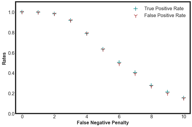
We see that as we increase the penalty, we lower both rates. This lowers our overall risk, but comes at the expense of missing more true positive (borrowers we should have invested in). We would prefer to decide on a model that has a true positivity rate higher than the false positivity rate.
Next, we tried using a Random Forest to see if a different model would perform better. However, both the true positivity rate and the false positivity rate were very close to 1 for a variety of weights.
Next Steps
We conclude that our logistic regression model performed the best. The exact model would depend on the level of risk that we found acceptable. Some possible next steps if we wanted to improve this more would be:
- test other classification models such as XGBoost or KNN
- hyperparameter tuning of the model (including the weights)
- fine-tuning the cross validation to ensure a balance of loan outcomes in each data fold
- take a closer look at the features to see if there are any we could remove or if we could engineer new features