Predicting Bike Rentals
See the full Jupyter Notebook on GitHub.
Many U.S. cities have communal bike sharing stations where you can rent bicycles by the hour or day. Washington, D.C. is one of those places, and collects detailed data on the number of bicyles people rent by the hour and the day.
Data Set
This data contains 17380 rows, with each row representing the number of bike rentals for a single hour of a single day. The data can be downloaded from the UCI Machine Learning Repository. The relevant columns are:
instant- A unique sequential ID number for each rowdteday- The date of the rentalsseason- The season in which the rentals occurredyr- The year the rentals occurredmnth- The month the rentals occurredhr- The hour the rentals occurredholiday- Whether or not the day was a holidayweekday- The day of the week (as a number, 0 to 7)workingday- Whether or not the day was a working dayweathersit- The weather (as a categorical variable)temp- The temperature, on a 0-1 scaleatemp- The adjusted temperaturehum- The humidity, on a 0-1 scalewindspeed- The wind speed, on a 0-1 scalecasual- The number of casual riders (people who hadn’t previously signed up with the bike sharing program)registered- The number of registered riders (people who had already signed up)cnt- The total number of bike rentals (casual + registered)
Goal
Build a machine learning pipeline that will predict the total number of bikes people rented in a given hour. We will use the cnt column as our target column, and decide which columns to use except for casual and registered.
Data Exploration
To start, we perform some simple data exploration to preview the data and begin to understand our target feature. First, we make a histogram of the CNT column.
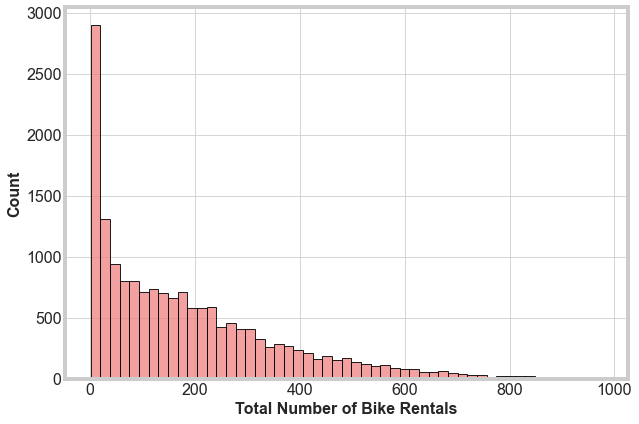
We see that this histogram is heavily right-skewed. Most of the total rentals per hour is low, less than about 100, but there is a long tail up to around 800. Second, we run a quick correlation for each column with the target column. We get:
| Column Name | Correlation Coefficient |
|---|---|
| season | 0.178 |
| yr | 0.250 |
| mnth | 0.120 |
| hr | 0.394 |
| holiday | -0.030 |
| weekday | 0.026 |
| workingday | 0.030 |
| weathersit | -0.142 |
| temp | 0.404 |
| atemp | 0.400 |
| hum | -0.322 |
| windspeed | 0.093 |
There are a range of correlation coefficient, unsurprisingly, with none higher than about 0.4.
Feature Engineering
Let’s engineer a new features that are more relevant and helpful for our pipeline.
The hr column contains the hours bikes are rented, from 1 to 24. Let’s create a new column, grouping these hours by morning, afternoon, evening, and night. We write a simple function to do this
def assign_label(value):
    if value >= 6 and value < 12:
        return 1
    elif value >= 12 and value < 18:
        return 2
    elif value >= 18 and value < 24:
        return 3
    elif value >= 0 and value < 24:
        return 4
then use the series.apply method to create the new column
bike_rentals['time_label'] = bike_rentals['hr'].apply(assign_label)
Split Data into Train and Test Sets
We’re ready now to split the data into train and test sets. We’ll start with using 80% of the data to train. Later, we’ll use cross-validation to improve our testing. We’ll use the mean squared error metric makes the most sense to evaluate our error. MSE works on continuous numeric data, which fits our data quite well. We are going to test a few different models first to check performance before deciding on the best method.
Linear Regression
We’re now ready to start fitting models to the data. We will start with a linear regression model. Linear regression works best when features are linearly correlated with the target and independent.
With the sklearn Linear Regression model, we get a mean squared error of 17154. This is a very high MSE. This is likely a result of the fact that the cnt column has a large number of small rentals. Missing these values significantly would increase the MSE quickly.
Decision Tree
Next, let’s try a decision tree regressor. We can compare this to the linear regression model to decide on the best algorithm for this dataset.
With the sklearn Decision Tree Regressor, we get a mean squared error of 2498. Our error has improved significantly.
Random Forest
Finally, lets try a random forest algorithm. With the sklearn Random Forest Regressor we get a mean squared error of 1617. Unsurprisingly, the random forest algorithm performs the best between the three models. Let’s focus on this model to refine the features to use and hyperparameters.
Feature Selection
We briefly looked at correlations between features and the target. Now, let use those to see if dropping any features can improve our model. We will first build a test and train function to quickly test our selections, and include cross-validation. At this point, we will use the default setting on the RandomForestRegressor. In the next step we will tune these parameters.
In our first step of feature selection, we drop a single column at a time and compute the MSE. This is a quick way to identify columns that play an outsized role in accuracy. We find that dropping any individual column provides little increase in the accuracy of our model.
The second quick step is to calculate the mutual information between each column and the target. We plot the results visually:
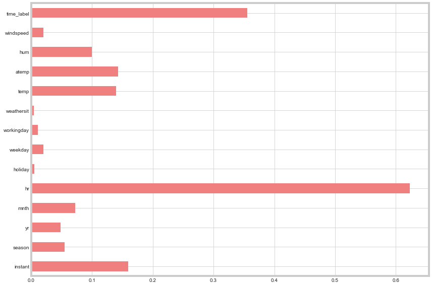
Windspeed, weathersit, workingday, weekday, and holiday have very little mutual information. Unsurprisingly, these columns also have limited correlation values with the target column. Dropping all of these features increased the error significantly. Though the mutual information on each individual feature is low, collectively they appear to provide important information we’ll keep.
Hyperparameter Testing
Now that we have selected our features, we can move to fine tuning our random forest parameters. For this, we’ll conduct a randomized grid search across possible parameters before fine-tuning our choices.
We set up a grid of parameters to test, then we use RandomizedSearchCV to search through the grid, using cross-validation to identify the best hyperparameters. Though we are considering 6 variables, we can plot slices through two parameters as a heatmap to get a sense of the parameter space.
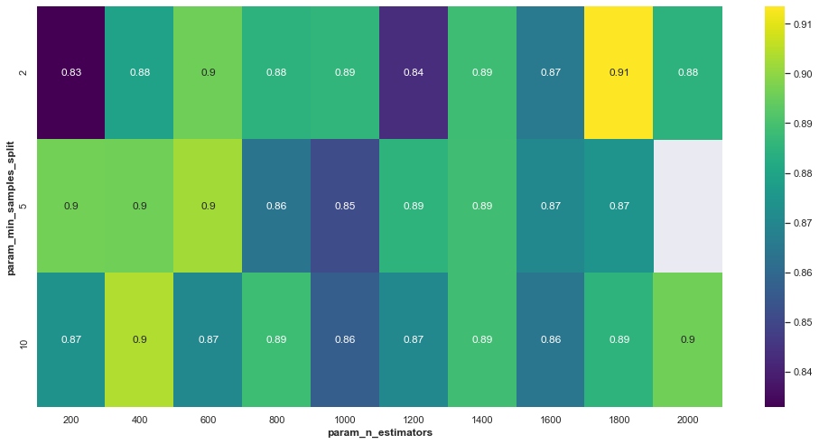
Though there not a large difference in the parameter space we plot here, a few percentage point difference makes a large difference when applied to larger datasets.
Final Model
Finally, we run the random forest with the features and hyperparameters we selected in the previous two steps and use cross-validation to get a final mean squared error of 1643, which is the best we have achived.