Predicting the Stock Market
See the full Jupyter Notebook on GitHub.
In this project, we will work with data from the S&P500 Index. We will use historical data to make predictions about future behavior.
Data
Our data covers the years 1950 to 2015. Each row in the file contains a daily record of the price of the S&P500 index. The columns in the dataset are:
Date– The date of the record.Open– The opening price of the day (when trading starts).High– The highest trade price during the day.Low– The lowest trade price during the day.Close– The closing price for the day (when trading is finished).Volume– The number of shares traded.Adj Close– The daily closing price, adjusted retroactively to include any corporate actions.
Goal
We will train the predictive model we build using data from 1950-2012 and make predictions from 2013-2015.
Data Cleaning
The Date column is an object type. Let’s go ahead and convert it to a datetime type using pd.to_datetime. This will allow us to more easily extract specific date ranges.
We also note that dates are sorted reverse chronologically, starting with the last day (2015) and moving towards earlier dates. Let’s sort this in ascending order instead.
index.sort_values(by='Date',ascending=True,inplace=True)
Generating Indicators
Since we have time series data, let’s generate a few indicators to make our model more accurate. We’ll create a few of these, but will need to be careful. Stock market data is sequential and each observation comes a day after the previous observation. Thus, the observations are not all independent. We don’t want to inject future knowledge into past row when we train and predict. For example, when creating an average price from the last 5 days we do not want to include the current day in that average. We’ll create the following indicators:
- average closing price from the past 5 days
- average closing price from the past 30 days
- average closing price from the past 365 days
- ratio between the average price from the past 5 days and the average price from the past 365 days
- average volume from the past 5 days
- average volume from the past 30 days
- average volume from the past 365 days
- standard deviation of the closing price from the past 5 days
- standard deviation of the closing price from the past 30 days
- standard deviation of the closing price from the past 365 days
- standard deviation of the volume from the past 5 days
- standard deviation of the volume from the past 30 days
- standard deviation of the volume from the past 365 days
We will use the rolling function in pandas to accopmlish this. However, the rolling mean will use the current days price, so we need to reindex the series to shift all the values forward one day.
An example of this is done with
index['avg_close_5'] = index.Close.rolling(5).mean().shift(periods=1)
And to create our ratios, we will use the np.where function because we need to easily account for the NaNs, such as
index['avg_close_ratio'] = np.where(index['avg_close_365'] != np.nan, index['avg_close_5'] / index['avg_close_365'], np.nan)
Splitting Up the Data
Since we generated some indicators, there are some rows where there is now missing data. We’re going to drop these data. While this means we’ll drop about a years worth of data, because of the 365 day average, the training set is large enough that this is only about 1.5% of the total data.
Now we are ready to split the data into the training set and the testing set. Dates before 2013-01-01 will go into the training set and dates after that will go into the testing set. We can use the datetime module to make this easy:
train = index[index['Date'] < datetime(year=2013,month=1,day=1)]
test = index[index['Date'] >= datetime(year=2013,month=1,day=1)]
Making Predictions
We are now ready to build our model. We will use a simple Linear Regression model from sklearn. We will use mean absolute error as the metric because it is very simple to understand in this situation. We will only use our generated indicators for the training and testing because the original columns all have some data leakage issues.
We also try dropping individual indicators to see if any make a significant change on the result. The mean absolute error is surprising insensitive to dropping most of these columns with the exception of avg_close_5, the average closing from the previous 5 days. Dropping the other columns produces very little change.
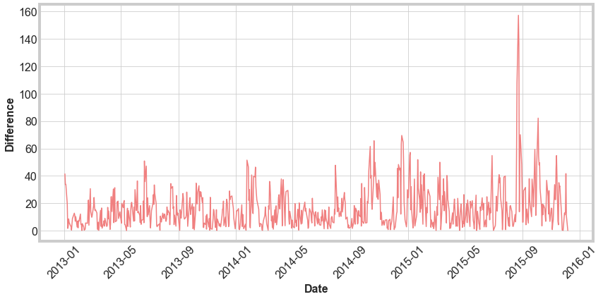
Finally, we calculate the difference for each data and plot to visualize. The final mean absolute error of 16 is not terrible, but there is a lot of flucuation in the results. To improve the model, we could consider adding in the day of the week..

Daily Predictions
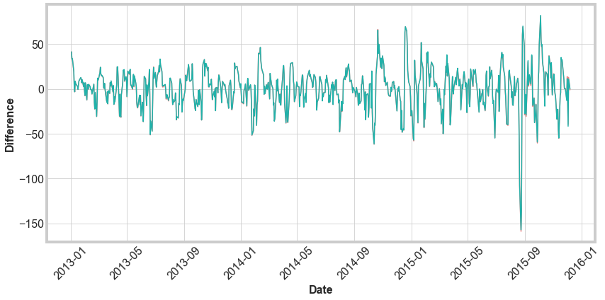
Finally, we update our pipeline to make a single daily prediction at a time. We will use all the data until the day before to make our prediction, so the training set gets larger as the we make later and later predictions. We still use the full set of features we used before. Below is a comparison between the difference in the predicted closing price and actual closing price for the mass predictions (green) and the daily prediction (red).

We see that there is basically no difference in the accuracy of the predictions. The difference in these methods is extremely negligible. So the additional training data does not increase model accuracy. As a next step, we could add the day of the week, as mentioned above. Another alternative would be to weight more recent data stronger than less recent data. This would be somewhat complicated to do and we would need to attempt it very carefully.