Euro Exchange Rates
Introduction
We will explore the daily Euro exchange rates between 1999 and 2021. The dataset is available on Kaggle.
This project is mostly a data visualization exercise, so we will mostly focus on the two final outcomes we produced. We will only briefly mention some noteworthy information about the dataset.
You can find the full Jupyter Notebook on GitHub here.
Data
This dataset contains 5699 rows and 41 columns. Most of the values are stored as objects. The first column (Period\Unit) lists the date. Every other column gives the exchange rate for that day to 40 other currencies. Most of the exchanges rates have minimal missing data, with the exception of:
- Cypriot pound
- Estonian kroon
- Greek drachma
- Iceland krona
- Lithuanian litas
- Latvian lats
- Maltese liras
- Slovenian tolar
- Slovak koruna
The majority of these countries are currently in the EU and use the Euro, so we lose their exchange rate data when they switch.
To clean the data, we do the following:
- We rename the columns to something easier to type
- We change the Time column to a datetime data type.
- We sort the values by Time in ascending order.
- We reset the index (and drop the initial index).
- Drop any rows that do not have exchange rate data for the currencies we are interested in.
- Perform a rolling mean to smooth out the data as both of our visualizations look at rates over a longer period of time.
Data vis 1: Exchange Rate by US President and UK Prime Minister
Show how the Euro-US dollar rate changed over the three previous presidents and five previous UK prime ministers.
- Bush (2001 - 2009)
- Obama (2009 - 2017)
-
Trump (2017 - 2021)
- Blair (1997 - 2007)
- Brown (2007 - 2010)
- Cameron (2010 - 2016)
- May (2016 - 2019)
- Johnson (2019 - present)
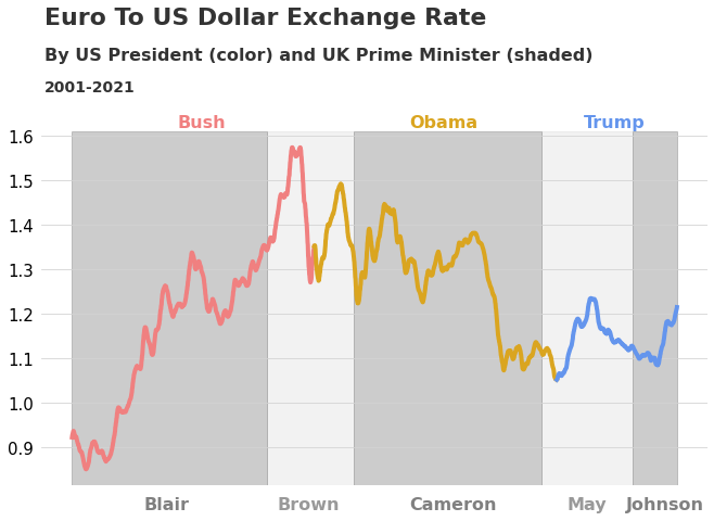
We wanted to find a way to illustrate the exchange rate over time as well as highlight the tenure’s of US Presidents and UK Prime Ministers. We think this figure does a pretty good job. Using different methods (colors vs shading) is a quick way to highlight the differences we are looking at without the graph getting too busy.
Year before joining EU
Now, let’s examine how the exchange rates changed in the last year for countries joining the EU.
The dataset runs from January 1999 until January 2021. From the EU website, here is the timeline of countries joining:
- January 5, 2004 - Czech Republic, Estonia, Cyprus, Latvia, Lithuania, Hungary, Malta, Poland, Slovakia, and Slovenia
- January 1, 2007 - Romania and Bulgaria
- January 7, 2013 - Croatia
Estonia has incomplete data, indicated by having a single, constant value. Therefore, we will drop Estonia from this analysis.
Poland, Bulgaria, and Lithuania are also missing data in the year before they joined, so we will exclude them as well.
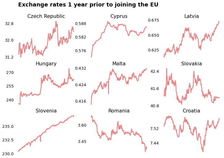
We used a simple 3x3 grid to create this figure. We had to keep y-axis labels so we had a point of reference for each country. This graph has the ability to communicate one more thing. We considered options, like adoption time of the Euro, but nothing added interesting information. Having different colored lines could do this quite simply.