Exploring Used Car Sales
Final Jupyter Notebook can be found here.
We’ll use data from eBay Kleinanzeigen, a classifieds section of the German eBay website. A few modifications have been made to the original dataset:
- 50,000 points have been sampled from the full dataset
- The dataset has been dirtied to test and improve data cleaning skills
Goal
Our goal is to create a clean data set and perform some basic analysis of the data.
Data Dictionary
dateCrawled- When this ad was first crawled. All field-values are taken from this date.name- Name of the car.seller- Whether the seller is private or a dealer.offerType- The type of listingprice- The price on the ad to sell the car.abtest- Whether the listing is included in an A/B test.vehicleType- The vehicle Type.yearOfRegistration- The year in which the car was first registered.gearbox- The transmission type.powerPS- The power of the car in PS.model- The car model name.kilometer- How many kilometers the car has driven.monthOfRegistration- The month in which the car was first registered.fuelType- What type of fuel the car uses.brand- The brand of the car.notRepairedDamage- If the car has a damage which is not yet repaired.dateCreated- The date on which the eBay listing was created.nrOfPictures- The number of pictures in the ad.postalCode- The postal code for the location of the vehicle.lastSeenOnline- When the crawler saw this ad last online.
Initial Data Exploration
We load the relevant libraries and load the dataframe as autos. We run autos.info() to view some basic information about the datset.
The majority of columns are stored as strings.
There are two columns that are stored as objects that we will want to convert to numerics: price and odometer. The price is an object because is begins with $. The odometer reading ends with km
There are five columns that have missing data. Sorted from least to most missing data: gearbox, model, fuelType, vehicleType, and notRepairedDamage
The dates are stored in YYYY-MM-DD format and the times are 24 hours.
The column names are stored in camelcase.
Cleaning Column Names
Let’s change the column name case to snake case. This will make them easier to read. We’ll run autos.columns to get a printed list of columns. We copy this list to a new list, updated the names as desired and save it to the dataframe using autos.columns = new_column_names
Identify Cleaning Tasks
To identify any columns that need cleaning, we start by running autos.describe(include='all') to see descriptive statistics for all columns.
seller and offer_type both are nearly uniform columns, with all values being the same with one exception.
As mentioned previously, price and odometer columns will need to be cleaned and converted to numerical values. The price is an object because is begins with $. The odometer reading ends with km.
Clean price and odometer columns
We’ll start by first cleaning the price columns. We need to remove the $ and , characters from the values. Then, we need to convert the column to a numeric datatype. We accomplish this with the following:
autos['price'] = autos['price'].str.replace('$','')
autos['price'] = autos['price'].str.replace(',','')
autos['price'] = pd.to_numeric(autos['price'])
We do a similar thing for the odometer column, but also want to rename the column so that we keep the units
autos['odometer'] = autos['odometer'].str.replace('km','')
autos['odometer'] = autos['odometer'].str.replace(',','')
autos['odometer'] = pd.to_numeric(autos['odometer'])
autos.rename(columns={'odometer':'odometer_km'}, inplace=True)
Explore price and odometer columns
Now that we have cleaned and converted these to numeric data types, let’s examine the values to see if there are any outliers. From autos['price'].unique().shape we find that there are 2357 unique values in our dataframe. We then use .describe() and .value_counts() to see some more details.
The upper quartile is at $7200. We could consider values over 1,000,000 an extreme outlier. This is only 11 vehicles, so would not significantly change our dataset.
On the other end, we have 1421 cars listed at a price of $0 and 1762 at < $100. These seem like very low prices for cars, so we’ll (somewhat arbitrarily) use this as a cutoff to remove extreme price outliers. There are only 445 values between 100 and 200, so we see that this number drops relatively quickly.
We now drop these rows using Boolean logic:
autos = autos[(autos['price'] > 100) & (autos['price'] < 1000000)]
We now look at the odometer_km column to similarly explore any unusual values. We use the same Pandas commands to perform this analysis. The odometer column does not seem to have any unusual outliers. All values are one of 13 unique values, between 5000 and 150000. This seems reasonable since we are dealing with used cars. Reported values must be rounded to the nearest 10- or 25-thousand miles.
Exploring the Date Columns
Let’s explore the date columns to understand the date ranges this data covers. There are 5 columns related to dates. Three of those are currently stored as strings, so we need to convert into numerical representation so that we can analyze it. We can create a distribution of dates by extracting those using
autos['date_crawled'].str[:10].value_counts(normalize=True,dropna=False)
Here, we also normalized the values and told Pandas to include missing values. We can do some exploratory analysis on the date_crawled, ad_created, and last_seen columns.
The majority of these dates come from 2016. The crawler was only run in March and April of 2016. Thus, the date_crawled and last_seen columns have similar ranges of dates.
The ads were created between June of 2015 and April of 2016.
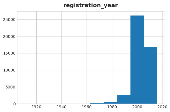
Now, let’s take a look at the registration years of the cars. The mean registration year is 2004, with a wider range of standard deviations of 88 years. This indicates that there are a decent number of older cars. However, we also see that the minimum year is 1000 and the max year is 9999. So there is some incorrect data for the registration years that we’ll need to deal with.
The first production of automobiles in Germany was late 1800s, so we can use 1900 as a cut-off.
At the other end, the crawler was run in 2016, so we should not find cars with registration years later than that. There are about 2500 autos with 2017 and 2018 registrations listed, which could be typos. Values larger than that should definitely not be used for analysis.
We will use 1900-2016 as the range of acceptable values. The number of autos we lose from 2017 and 2018 are relatively small.
We drop these values using Boolean logic again
autos = autos[(autos['registration_year'] > 1900)
              & (autos['registration_year'] < 2017)]
And we can use Seaborn to plot a histogram of years. We see that there are very few cars that were first registered before 1960, which makes sense.
Exploring Price By Brand
Let’s now explore price based on brand. We have quite a few different brands included in our data, so for simplicity we’ll need to break this down. When we look at the normalized value counts by brand, we decide to focus on only those brands that account for at least 1% of the total values.
In order to determine the mean price by brand, we will create a new dictionary with this information. We start with a list of the brands we are interetsed in, then loop through that list.
brand_list = ['volkswagen', 'bmw', 'opel', 'mercedes_benz', 'audi', 'ford', 'renault',
       'peugeot', 'fiat', 'seat', 'skoda', 'nissan', 'mazda', 'smart',
       'citroen', 'toyota', 'hyundai']

brand_dict = {}

for x in brand_list:
    short_auto = autos[autos['brand'] == x]
    mean_price = short_auto['price'].mean()
    brand_dict[x] = mean_price
This is quite a few to look at in a table, so we create a plot to visualize this.
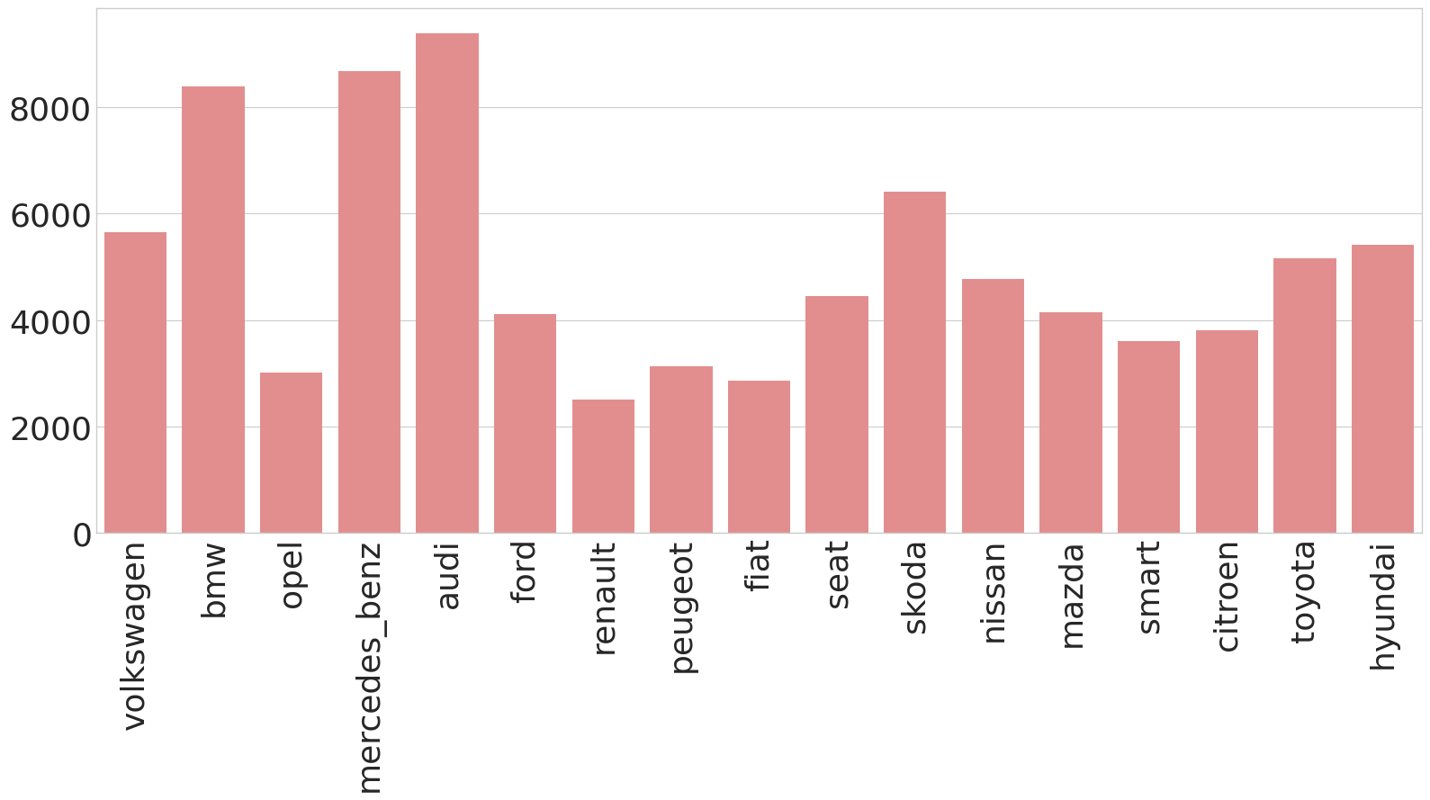
We see that BMW, Mercedes Benz, and Audi have the highest mean price by quite a lot.
Finally, let’s look at only the top 6 brands: Audi, BMW, Mercedes Benz, Ford, Opel, and Volkswagen. Let’s use aggregation to understand the average mileage for those cars and see if there’s any link with mean price. We use similar code as above to calculate the mean price and the mean mileage separately. Now, we need to combine these dictionaries. To do this, we convert them to a Pandas Series and build a new dataframe.
price_series = pd.Series(short_brand_dict)
mileage_series = pd.Series(short_mpv)

df = pd.DataFrame(price_series, columns=['mean_price'])
df['mean_mileage'] = mileage_series
| Mean Price | Mean Mileage | |
|---|---|---|
| Volkswagen | 5656 | 128787 |
| BMW | 8384 | 132716 |
| Opel | 3019 | 129379 |
| Mercedes-Benz | 8674 | 131053 |
| Audi | 9389 | 129260 |
| Ford | 4114 | 124249 |
The mean mileage is pretty similar to each other for these top six brands. This indicates that the difference in price is likely caused by inherent differences in the starting price point.