Predicting Energy Generation Pricing and Load

You can view the completed Jupyter Notebook on GitHub.

For this project, we are going to use the Hourly Energy Demand Generation and Weather dataset on Kaggle to look at energy prices and load. Energy forecasting has been described as one of the major fields where machine learning can have a significant impact. This data set contains 4 years of electrical consumption, generation, pricing, and weather from Spain. It is split into two data sets, energy and weather.

Goal

The goals of this project will be to

• clean and combine the data sets
• build a machine learning pipeline that can predict the energy price
• build a machine learning pipeline that can predict the load

Data Dictionary

For the energy dataset:

• time: Datetime index localized to CET
• generation biomass: biomass generation in MW
• generation fossil coal-derived gass: coal/lignite generation in MW
• generattion fossil coal-derived gass: coal/gas generation in MW
• generation fossil gass: gas generation in MW
• generation fossil hard coal: coal generation in MW
• generation fossil oil: oil generation in MW
• generation fossil oil share: shale oil generation in MW
• generation fossil peat: peat generation in MW
• generation geothermal: geothermal generation in MW
• generation hydro pumped storage aggregated: hydro1 generation in MW
• generation hydro pumped storage consumption: hydro 2 generation in MW
• generation hydro run-of-river and poundage: hydro 3 generation in MW
• generation hydro water reservoir: hydro 4 generation in MW
• generation marine: sea generation in MW
• generation nuclear: nuclear generation in MW
• generation other: other generation in MW
• generation other renewable: other renewable generation in MW
• generation solar: solar generation in MW
• generation waste: waste generation in MW
• generation wind offshore: wind offshore generation in MW
• generation wind onshore: wind onshore generation in MW
• forecast solar day ahead: forecasted solar generation
• forecast wind offshore eday ahead: forecasted offshore wind generation
• forecast wind onshore day ahead: forecasted onshore wind generation
• total load forecast: forecasted electrical demand
• total load actual: actual electrical demand
• price day ahead: forecasted price in EUR/MWh
• price actual: price in EUR/MWh

And for the weather dataset:

• dt_iso: datetime index localized to CET
• city_name: name of city
• temp: in Kelvin
• temp_min: minimun in K
• temp_max: maximum in K
• pressure: pressure in hPa
• humidity: humidity in percent
• wind_speed: wind speed in m/s
• wind_deg: wind direction
• rain_1h: rain in last hour in mm
• rain_3h: rain in last 3 hours in mm
• snow_3h: snow in last 3 hours in mm
• clouds_all: cloud cover in percentage
• weather_id: code used to describe weather
• weather_main: short description of current weather
• weather_description: long description of current weather
• weather_icon: weather icon code for website

Load and Preliminary Explore the Data

As always, we will start by load and doing a preliminary exploration of the data. We can use some of our standard Pandas commands to do this, including df.dtypes, df.isnull().sum(), and series.nunique()

Energy Data Set

The energy data set has 29 columns and 35,064 rows. All columns are float except for the time column. We should convert that column to a datetime object so we can more easily use the times. Most columns have less than 20 missing values. However, two columns (generation hydro pumped storage aggregated and forecast wind offshore eday ahead) are missing all values. We should remove those columns. A few additional columns have only a single unique value (typically 0). We will remove these columns (generation fossil coal-derived gas, generation fossil oil shale, generation fossil peat, generation geothermal, generation marine, and generation wind offshore) because they do not provide any helpful information.

Finally, we note that the column names have spaces between the words. To make it easier for our coding, we’ll replace the spaces with underscores.

Data cleaning tasks for the energy data set:

• convert the time column to a datetime object
• remove generation hydro pumped storage aggregated and forecast wind offshore eday ahead
• remove generation fossil coal-derived gas, generation fossil oil shale, generation fossil peat, generation geothermal, generation marine, and generation wind offshore
• replace spaces in column names with underscore

Weather Data Set

Now, let’s explore the weather data set so we understand the data structure and any data cleaning tasks.

The weather data set has 17 columns and 178,396 rows. It is very clean. There are no null values and every column has multiple unique values. There are data included for five cities: Madrid, Bilbao, Seville, Barcelona, and Valencia. Barcelona has a leading space at the beginning that we’ll have to be careful with. Each city is included a different number of times, so we’ll have to sort out why that is. There are 35,064 unique datetimes. That matches the number in the energy dataset. Hopefully all of these match, but we’ll have to check first. The majority of the columns are numeric types. The weather_main, weather_description, and weather_icon are all objects. These could be useful as a general description of the type of weather, so we will keep all of these for now.

Data cleaning tasks for the weather data set:

• convert dt_iso to a datetime object

Data Cleaning

Now that we have explored and identified what we need to do for data cleaning, let’s implement it for both data sets.

For the energy data set, we use the following code:

energy['time'] = pd.to_datetime(energy['time'])

columns_to_remove = ['generation hydro pumped storage aggregated','forecast wind offshore eday ahead',
                    'generation fossil coal-derived gas','generation fossil oil shale',
                    'generation fossil peat','generation geothermal',
                    'generation marine','generation wind offshore']

energy_clean = energy.drop(columns_to_remove,axis=1)

energy_clean.columns = energy_clean.columns.str.replace(' ','_')

and for the weather data set, we simply use

weather['dt_iso'] = pd.to_datetime(weather['dt_iso'])

Merging Data

Now that both data sets have been cleaned, we are ready to merge them into a single dataframe.

First, we need to find out if the times in both data sets are the same. The times in weather are repeated, so we need to extract the unique times first.

weather_unique_times = weather['dt_iso'].unique()
energy_unique_times = energy_clean['time'].unique()

Then we can create a Boolean array to see if the times match. This assumes they start and end at the same time, but is the simplest place to start

test_times = weather_unique_times == energy_unique_times

Then, we count the number of False values and find 0, indicating the the times in both data sets match.

Now, we want to fold the weather data set into the energy data set. We want to separate out the weather data by city, then add each relevant column. We should prepend the name of each city to the feature on the new data set, such as madrid_temp. If we do this, we will have a single row per time stamp with all relevant data. The following block of code will accomplish this:

city_names = ['Madrid','Bilbao','Seville',' Barcelona','Valencia']

# let's create an iteration variable so we don't overwrite our data
# we'll use this instead of looking for Madrid so our code is more flexible
iteration = np.linspace(1,len(city_names),num=len(city_names))

# now we loop through cities and the iteration variable to create
# the new, merged dataframe

for city, it in zip(city_names,iteration):
    # extract only the city for this iteration
    city_extract = weather[weather['city_name'] == city]
    
    # alter the names of the columns to suffix the name of the city
    if city == ' Barcelona':
        city = 'Barcelona' # remove the leading space
    city_suffix = '_' + city
    city_extract = city_extract.add_suffix(city_suffix)
    city_time_col = 'dt_iso_' + city
    
    # merge the dataframes. the first time we need to name the
    # new dataframe, then we don't want to overwrite it
    
    if it == 1:
        full_df = energy_clean.merge(city_extract,
                                    left_on='time',right_on=city_time_col,
                                    how='left',suffixes=(None,city))
    else:
        full_df = full_df.merge(city_extract,
                                left_on='time',right_on=city_time_col,
                                how='left',suffixes=(None,city))
        

After checking that the times in the new dataframe match, we drop the times for each city.

Visualizing the Data Set

Now that we have cleaned and merged the data sets, let’s do a few simple visualizations so that we can better understand the type and distributions of data we have.

We’ll start off with a histogram of each generation type. The range of each type varies quite significantly. They each have different levels of normal and skew. Three appear as if they have a large number of zero or near-zero values.

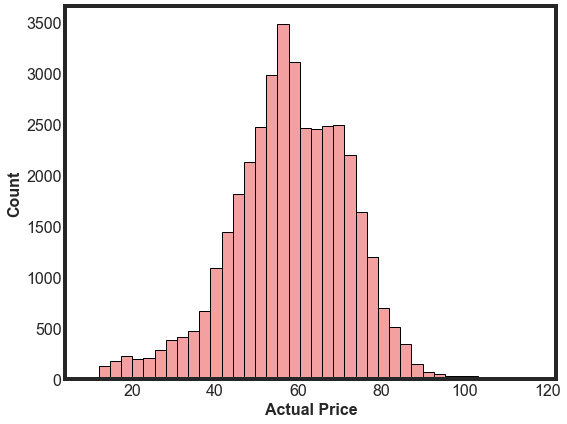
Next, let’s take a look at the Actual Price column. This column will be one of our target values when we build our machine learning model below. It’s good practice to visualize the distribution of target values. This distribution looks very close to normal and there are not a lot of outliers, which is great.

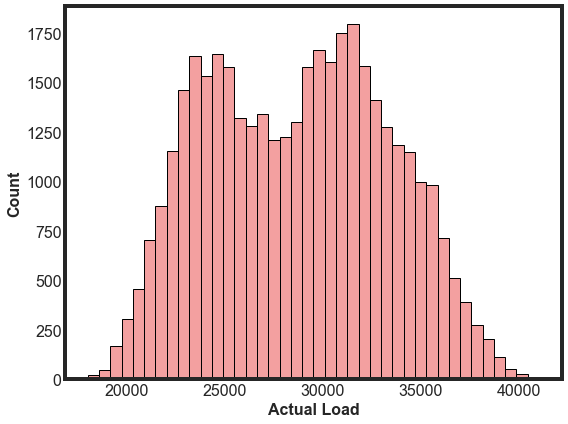
Next, let’s look at the Actual Load distribution. We will also build a model to predict the load based on the weather. This distribution is dual peaked and there are no significant outliers.

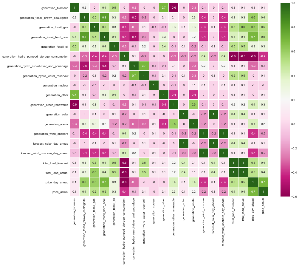
Finally, let’s look at a couple of heatmaps to get an initial sense of collinearity and correlations with our target variables. Unsurprisingly, there is a large amount of data leakage between the forecast and actual values. And there are a few generation types related to hydro display strong collinearity.

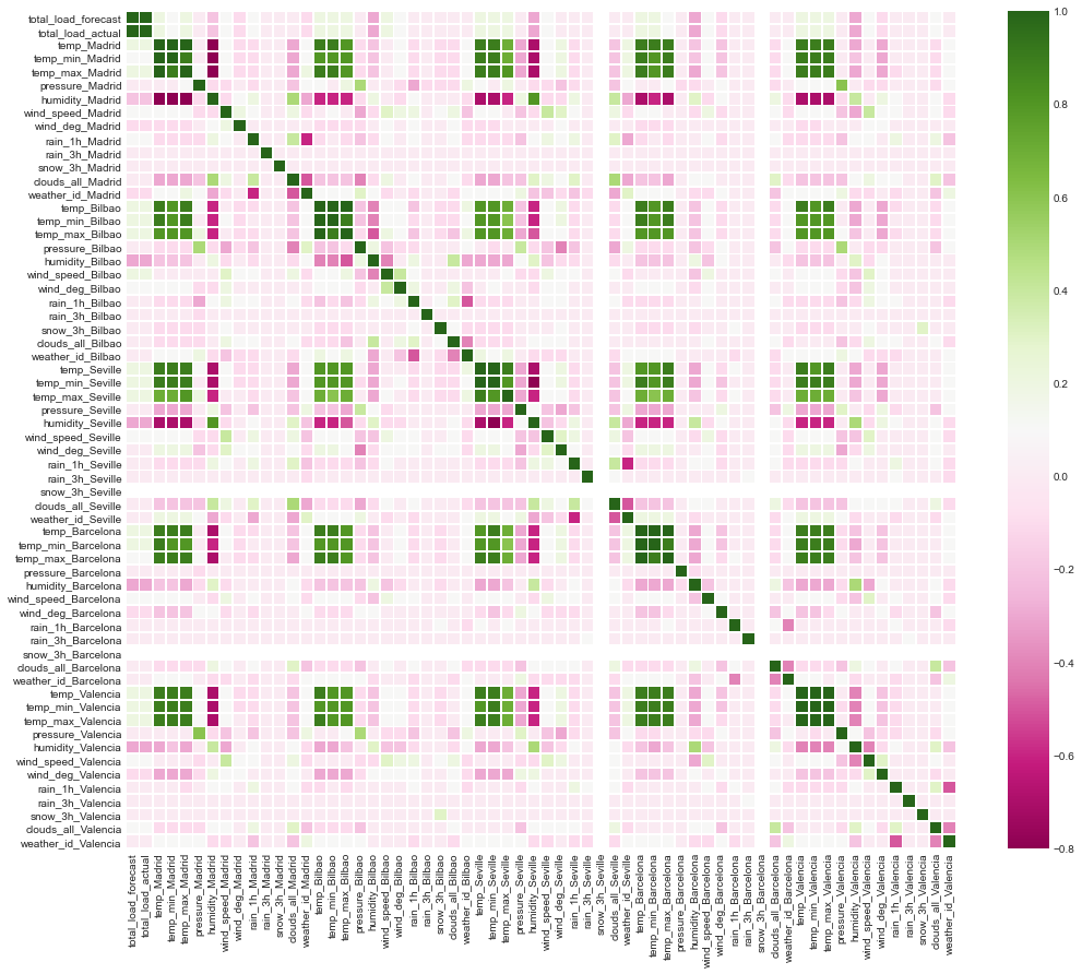
We’ll also look at a heatmap for the weather variables. There is a high correlation between the temperatures in each city. This is not surprising as Spain is a relatively small county, so we would not expect drastic temperature differences. We will want to be careful with these when we build and validate our pipeline.

Engineering Season

Let’s add a column for season. Season will be a better indicator of load and price than exact days or times. We’ll create a new column with four categorical values (winter, spring, summer, and fall). We could go ahead and encode these numerically, but for fun we’ll save this as a step for our pipeline to do later. We can use the following function to accomplish this:

def add_season(df,datetime_column):
    '''
    function to add season as a column to the dataframe
    
    INPUT:  df: dataframe with a datetime column 
            datetime_column: string, column with datetime values to classify the season
            
    OUTPUT: df: dataframe with new column season with values winter, spring, summer, or fall
    '''
    condition_winter = (df[datetime_column].dt.month>=1)&(df[datetime_column].dt.month<=3)
    condition_spring = (df[datetime_column].dt.month>=4)&(df[datetime_column].dt.month<=6)
    condition_summer = (df[datetime_column].dt.month>=7)&(df[datetime_column].dt.month<=9)
    condition_fall = (df[datetime_column].dt.month>=10)@(df[datetime_column].dt.month<=12)
    
     # Create column in dataframe that inputs the season based on the conditions created above
    df['season'] = np.where(condition_winter,'winter',
                            np.where(condition_spring,'spring',
                            np.where(condition_summer,'summer',
                            np.where(condition_fall,'fall',
                                     np.nan))))

    return df

Predicting Price

First, we are going to use this dataset to predict the price of energy. We will not include the full dataframe that we currently have; the weather is not going to change the predicted price. We will also remove the time column as we will not do any real-time forecasting at this point.

Our pipeline will need to accomplish a few different tasks:

• imputation - some of our columns have missing values. The majority are missing only 12-14 values, out of the 38568 rows we have. Since we are missing so few, we’ll impute values with SimpleImputer
• encoding of categorical values - when we added the season column, we decided to leave it as categorical. We will need to encode these values to numerical for the modeling.
• scaling - looking back at the histogram of generation values above, we see that there is a fairly wide range of possible values that differ by generation type. We’ll scale these so that they are more similar, which should improve our accuracy. We will try a few different options, including StandardScaler, MinMaxScaler, and MaxAbsScaler.
• feature selection - we have 15 different features we are using to make our predictions. This is not a terribly large number, but each feature might not be helpful for our modeling. We will try a few different feature selection algorithms to help us utilize only the most relevant features. We’ll try SelectKBest and Variance Threshold.
• model selection - finally, we will want to examine a few different models to select which one is best. We will start with comparing KNeighborsRegressor , RandomForestRegressor, and XGBRegressor.

After creating lists for the features and target column names, we create our relevant dataframes and use train_test_split to split the dataframe

X = energy_weather[predicting_price_features]
y = energy_weather[target]

X_train, X_test, y_train, y_test = train_test_split(X,y, test_size=0.2,random_state=0)

Then we build our pipeline using the following code block. We first have to separate the numerical and categorical columns since we will treat those differently in our preprocessor before we use GridSearchCV to test different feature selection algorithms and models.

num_cols = X_train.select_dtypes(exclude=['object']).columns.tolist()
cat_cols = X_train.select_dtypes(include=['object']).columns.tolist()

numeric_transformer = Pipeline(
    steps=[("imputer", SimpleImputer(strategy="median")), ("scaler", StandardScaler(with_mean=False))]
)

categorical_transformer = OneHotEncoder(handle_unknown="ignore")

preprocessor = ColumnTransformer(
    transformers=[
        ("num", numeric_transformer, num_cols),
        ("cat", categorical_transformer, cat_cols),
    ]
)

pipe = Pipeline(
    steps=[("preprocessor", preprocessor), 
           ('selector', VarianceThreshold()),
           ("regressor", KNeighborsRegressor())]
)

parameters = {'selector': [SelectKBest(), VarianceThreshold()],
              'regressor': [KNeighborsRegressor(),RandomForestRegressor(),XGBRegressor()]
}

grid = GridSearchCV(pipe, parameters, cv=3, scoring='neg_mean_absolute_error').fit(X_train, y_train)

print('Training set score: ' + '{:.4f}'.format(float(grid.score(X_train, y_train))))
print('Test set score: ' + '{:.4f}'.format(float(grid.score(X_test, y_test))))
print('Best model parameters: ' , grid.best_params_)

With this pipeline we get a training negative mean absolute error of -1.05 and a test error of -2.77 with the best model using VarianceThreshold and RandomForestRegressor.

During testing, we found that adding in the season increased the errors by a few percent.

Now that we have a baseline score, let’s try out a few different scaling methods. Since we have a preprocessor in our pipeline above, it’s a little more challenging to iterate over a few different scaling approaches. Instead, let’s write a for loop to iterate over the scaling types, then save the results to a dictionary that we can compare afterwards.

scaling_list = [StandardScaler(with_mean=False), MinMaxScaler(), MaxAbsScaler()]
scaling_dict = {}

num_cols = X_train.select_dtypes(exclude=['object']).columns.tolist()
cat_cols = X_train.select_dtypes(include=['object']).columns.tolist()


for scaler in scaling_list:
    numeric_transformer = Pipeline(
                steps=[("imputer", SimpleImputer(strategy="median")), ("scaler", scaler)]
                )

    categorical_transformer = OneHotEncoder(handle_unknown="ignore")

    preprocessor = ColumnTransformer(
        transformers=[
            ("num", numeric_transformer, num_cols),
            ("cat", categorical_transformer, cat_cols),
            ]
            )

    pipe = Pipeline(
            steps=[("preprocessor", preprocessor), 
            ('selector', VarianceThreshold()),
            ("regressor", KNeighborsRegressor())]
            )

    parameters = {'selector': [SelectKBest(), VarianceThreshold()],
                'regressor': [KNeighborsRegressor(),RandomForestRegressor(),XGBRegressor()]
                }

    grid = GridSearchCV(pipe, parameters, cv=3, scoring='neg_mean_absolute_error').fit(X_train, y_train)

    train_score = grid.score(X_train, y_train)
    test_score = grid.score(X_test, y_test)
    best_model = grid.best_params_
    
    print('scaler: ', scaler)
    print('Training set score: ' + '{:.4f}'.format(float(train_score)))
    print('Test set score: ' + '{:.4f}'.format(float(test_score)))
    print('Best model parameters: ' , best_model)
    scaling_dict[scaler] = [train_score,test_score,best_model]

The scaling types had very little effect on the test scores. All three scaling types led to the same selector and regression model being selected (Variance Threshold and the Random Forest Regressor). Comparing the models with different scaling types:

Scaling Type	Best Score
Standard Scaler	-2.785
MinMax Scaler	-2.781
MaxAbs Scaler	-2.789

Predicting Load

Now we are going to use our weather-related information to predict the load. This is important for energy companies to ensure they have enough supply so that the grid does not collapse. We’ll note at the start that we expect our load predictions to be less accurate than our price predictions. This review of load forecasting found that, in general, 50% of the forecasted amounts depend on the weather and economics. We are only going to consider the weather at this point in time.

The snow columns for Seville and Barcelona have zero variance, so we will not include them here. The same for 3 hour rain total for Madrid.

Our pipeline will look similar to the one we built to predict the price, but there are a few differences we will want to take into account:

• We don’t have any missing values for the features, so we don’t need to impute any values.
• We have quite a few more features (55) than we had when we predicted price (16). Referring to the heat map above, there is a a lot of collinearity between these values. Feature selection will be more important than it was above.
• The target feature, total_load_actual, is missing 37 values, so we will need to remove those rows from the dataframe before modeling.

We use a very similar code block for this pipeline.

pipe_load = Pipeline([
    ('scaler', StandardScaler(with_mean=False)),
    ('selector', VarianceThreshold()),
    ('regressor', KNeighborsRegressor())
    ])

parameters_load = {'selector': [SelectKBest(), VarianceThreshold()],
                'regressor': [KNeighborsRegressor(),RandomForestRegressor(),XGBRegressor()]
                }

grid_load = GridSearchCV(pipe_load, parameters_load, cv=3, 
                         scoring='neg_mean_absolute_error').fit(X_train_load, y_train_load)

train_score_load = grid_load.score(X_train_load, y_train_load)
test_score_load = grid_load.score(X_test_load, y_test_load)
best_model_load = grid_load.best_params_

print('Training set score: ' + '{:.4f}'.format(float(train_score_load)))
print('Test set score: ' + '{:.4f}'.format(float(test_score_load)))
print('Best model parameters: ' , best_model_load)

And we get a mean negative absolute error for the training set of -814 and a test error of -2187.

There is a bit difference between our training scores and our test scores, about a factor of 3. This is probably an indication that we are overfitting our model. We are already doing cross-validation and using an ensemble model, which are two common ways to correct for overfitting.

We are currently including both the temperature (the meaning of which is unclear but is perhaps the average), the minimum temperature and the maximum temperature. There is a strong collinearity between these values. Let’s remove the min and the max from our feature list to ensure they are not being used for the predictions.

We tested the pipeline after removing these values and found not significant change in our final errors.

Conclusion and Next Steps

We predicted the price within about a mean absolute error of 2 points, compared to target values that approximately ranged between 20 and 80. For the mean value of 58, this corresponds to an error of about 3.4%

We predicted the load within about a mean absolute error of 2234, compared to target values that approximately ranged between 20,000 and 40,000. For the mean value of 28,738, this corresponds to an error of about 7.7%.

We are going to wrap up this project for now, but a few next steps we could take to improve our modeling performance could include:

• add information such as economic parameters, historical usage, and household lifestyle to the load predictions.
• categorize the days by month instead of year to add some granularity.
• use the original date times to forecast the price and load 24 hours in advance. We are currently predicting it instantaneously, but it would be more useful to predict both 24 hours in advance.
• tune the hyperparameters of the best feature selectors and models.

---

<

Previous Post

World Energy Consumption

>

Blog Archive

Archive of all previous blog posts