Predicting Car Prices with K-Nearest Neighbors
See the full Jupyter Notebook on GitHub.
Let’s practice the machine learning workflow to predict’s a car’s market price using its attributes. For each car in our dataset, we have information about the technical aspects of the vehicle, such as the weight of the car, the miles per gallon, the acceleration, etc. Our goal is to identify which of the attributes, or combination, is most helpful in predicting the price of a car. To do this, we’ll use K-Nearest Neighbors.
Data Set
We’ll be working with the Automobile Data Set from the UCI Machine Learning Repo.
The target column is Price.
The columns that are numeric are symboling, wheel-base, length, width, curb-weight, engine-size, compression-rate, city-mpg, and highway-mpg.
The are no missing values in any columns, though we note that in normalized-losses shown using cars.head() the first three values are ?, so we should be careful of missing values that are represented using other symbols.
Data Cleaning
Since we already noticed the data issue in the normalized-losses column, let’s replace the ? with a NaN. This might occur in other columns, so if we do this replacement across the whole dataframe, this can let us know which columns actually do have missing values.
cars.replace('?',np.nan,inplace=True)
We are only going to focus on continuous numeric data, so we need to select only those columns.
continuous_values_cols = ['normalized-losses', 'wheel-base', 'length', 'width', 'height', 'curb-weight', 'engine-size', 'bore', 'stroke', 'compression-rate', 'horsepower', 'peak-rpm', 'city-mpg', 'highway-mpg', 'price']
numeric_cars = cars[continuous_values_cols]
Then we convert all columns to float
numeric_cars = numeric_cars.astype('float')
and then check for null values
numeric_cars.isnull().sum()
There are four missing values in the price column. Since price is our target value, we will remove the rows with missing values.
We only have 205 rows, so want to preserve as much data as we can. So the remaining missing values we will fill with the mean from the column
numeric_cars = numeric_cars.fillna(numeric_cars.mean())
Let’s also rescale the values in the numeric columns so they all range from 0 to 1. Except for the Price column.
price_col = numeric_cars['price']
numeric_cars = (numeric_cars - numeric_cars.min())/(numeric_cars.max() - numeric_cars.min())
numeric_cars['price'] = price_col
Now that the data is clean, we are ready to build the model to make predictions.
Univariate Model
Let’s start with a simple univariate model. We will then use this to understand the features better when we build our multivariate model.
Let’s write a function that does the training and simple validation process.
def knn_train_test(df,training_col,target_col,k):
    # initialize the model and the folding for the
    # cross validation

    knn = KNeighborsRegressor(n_neighbors = k)

    kf = KFold(n_splits = 5, shuffle=True,random_state=1)

    # if we only want to check one column, we need to
    # convert it to a list
    if isinstance(training_col,str):
        training_col = [training_col]


    # use cross validation to determine the mse
    mses = cross_val_score(knn,
                       df[training_col],
                       df[target_col],
                       scoring='neg_mean_squared_error',
                       cv=kf)

    rmse = np.sqrt(np.absolute(np.mean(mses)))
    # return RMSE
    return(rmse)
Since we are starting with a Univariate model, we create a list of column names, and loop through them with our function, using the default value for k. We get the following results:
| Column Name | RMSE |
|---|---|
| engine-size | 3179 |
| horsepower | 3814 |
| highway-mpg | 4157 |
| width | 4241 |
| curb-weight | 4425 |
| city-mpg | 4502 |
| length | 5853 |
| wheel-base | 6155 |
| compression-rate | 6417 |
| bore | 6861 |
| normalized-losses | 7099 |
| stroke | 7134 |
| peak-rpm | 7599 |
| height | 7618 |
We then consider different values of k. For each individual feature, we five different k-values.
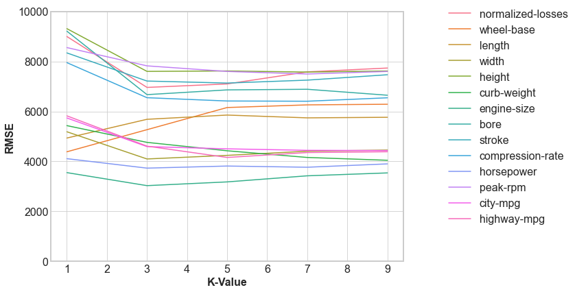
We see that while there is a change in the RMSE, only a few features change their order.
Multivariate Model
Now, let’s run some multivariate models so we can include multiple features. We will include the best two, three, four, and five features from the previous step to evaluate the impact of different features.
| Number of Features | RMSE |
|---|---|
| Two | 2994 |
| Three | 2862 |
| Four | 3166 |
| Five | 3159 |
Hyperparamater Tuning
Let’s now optimize the models that performed the best in the previous step. We’ll adjust the k value, the number of neighbors, from 1 to 25 for the three best models from above.
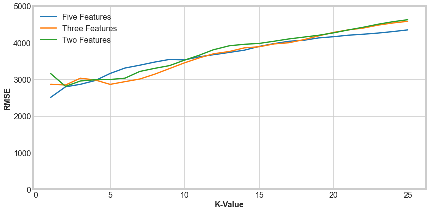
For the multivariate models, we see that the K-value we choose should be less than about 5. A k-value of 1 produces the least error for the Five features and Three features set. But a value of 1 would be prone to large errors for unusual cars, so we should avoid that. A value of 2 is most consistent for the lowest RMSE. There is only a small difference between the different models for k = 2. Five features has a slightly smaller error, and should perform better on outliers, so we would suggest using k = 2 with the five features we have used here.